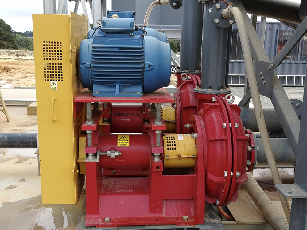
Introduction
A Pump curve chart is a graphical representation that illustrates the performance characteristics of a Pump. It provides information about how a Pump operates under different conditions, helping users to understand the Pump’s efficiency and capabilities. It is critical for Pump sizing and selection.
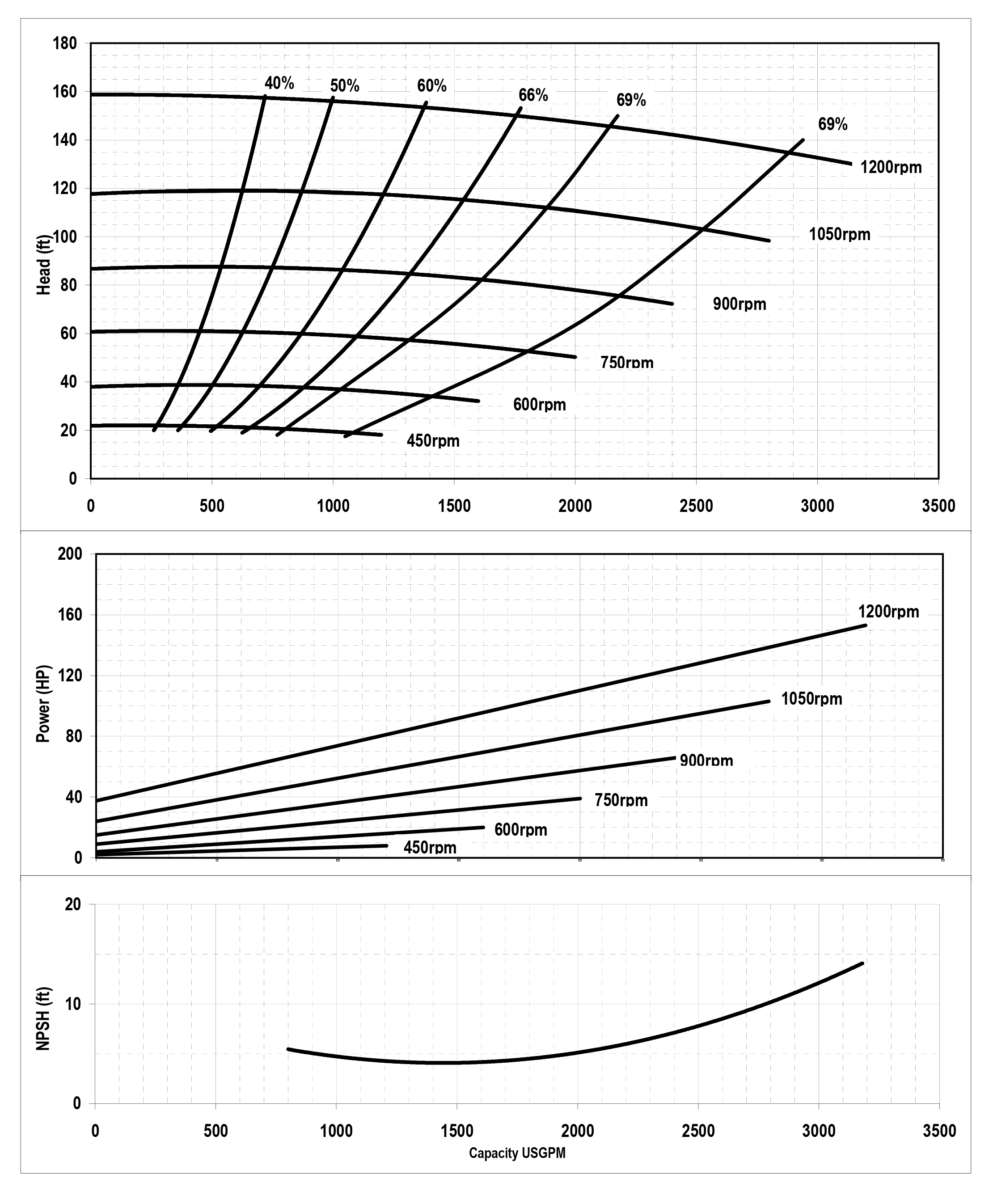
Pump curves have been around for a long time and contain a lot of information, including head, flow rate, efficiency and power consumption. A typical Pump curve contains four main data plots on an X-Y graph or graphs:
Total Dynamic Head
Total Dynamic Head (TDH) describes the total energy that a Pump must overcome to move a fluid from one point to another within a piping system. It is the sum of the following:
- Static head – the vertical distance between the surface of the liquid source and the Pump
- Pressure head – the pressure energy in the system, both suction (negative pressure) and discharge (positive pressure)
- Friction head – the energy lost due to the resistance encountered by the flowing fluid as it moves through the system
Total Dynamic Head is usually expressed in units of length, such as meters and feet. It is used to determine the Pump’s operating point, as the Pump must be capable of providing enough energy to overcome the TDH in the system to ensure proper fluid circulation.
Total Dynamic Head is depicted on the vertical Y-axis of the graph.
Flow rate
Flow rate refers to the volume of fluid the Pump is capable of moving through its system per unit of time. It is typically measured in gallons per minute (gpm), liters per second (L/s) or cubic meters per hour (m3/h).
The flow rate is influenced by the Pump’s ability to create a pressure difference, or head, that propels the fluid through the system. The Pump curve chart illustrates how the Pump’s flow rate changes at different levels of head.
Flow rate is depicted on the horizontal X-axis of the graph.
Power consumption
Power consumption is the amount of energy required for the Pump to operate at its duty point. It is typically measured in units of horsepower.
Power consumption is depicted on the vertical Y-axis of the graph.
Net Positive Suction Head required
Net Positive Suction Head required (NPSHr) is the minimum required pressure above the suction line to avoid cavitation issues at the selected flow rate. It is usually measured in feet or meters.
To avoid cavitation, the NPSHr should always be less than the Net Positive Suction Head available (NPSHa) provided by the sump. NPSHa represents the total suction head available at the Pump inlet and is calculated as the difference between the total suction head and the vapor pressure head. When the NPSHa is greater than NPSHr, the Pump is less likely to experience cavitation.
NPSHr is depicted on the vertical Y-axis of the graph.
Putting it all together
The Total Dynamic Head, flow rate, power consumption and NPSHr data, along with efficiency and speed ranges, are plotted on an X-Y graph called a Pump curve. The formatting of Pump curves may be different between manufacturers, but the principles of all Pump curves are the same. In some cases, the information is displayed on one graph with multiple vertical Y-axis labels (Total Dynamic Head, power consumption and NPSHr) and the flow rate depicted on the horizontal X-axis, as it is the common denominator.
In other cases, the information is displayed on three graphs: one depicting Total Dynamic Head and flow rate, another depicting power consumption and flow rate, and the third depicting NPSHr and flow rate.
As part of the graph(s), the speed range and efficiency points of the Pump are overlaid. The speed and efficiency information comes from extensive testing performed by the Pump manufacturer. This allows an individual to use their application’s Total Dynamic Head and flow rate to evaluate different Pumps to select the best option for their operation.
Once the Total Dynamic Head is determined and the desired flow rate is selected, it is an easy exercise to find information on the Pump Curve.
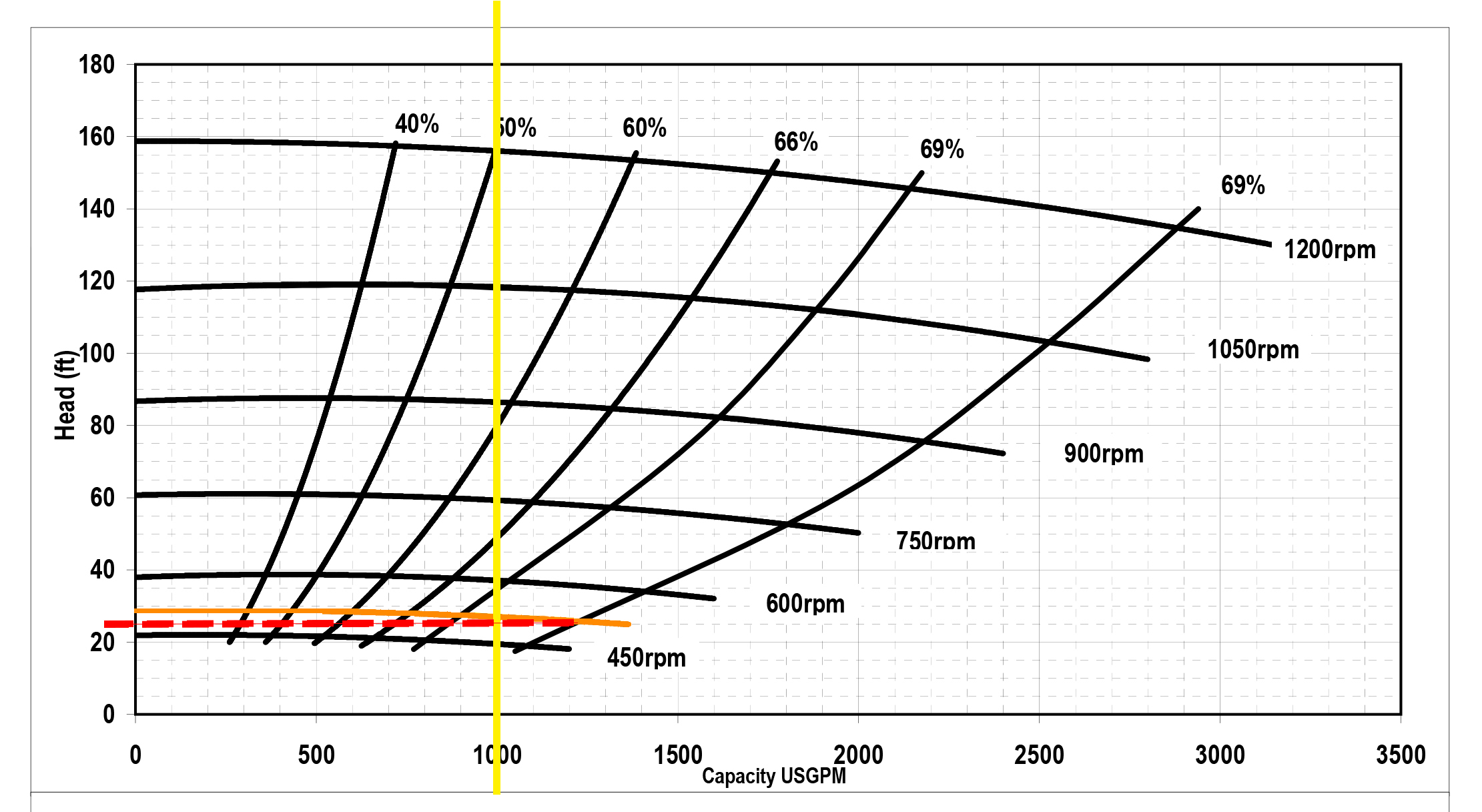
Consider a Pump curve with three graphs.
1. Find the duty point of the Pump
First, identify the axes on the graph depicting Total Dynamic Head and flow rate. The vertical axis (Y-axis) represents the Total Dynamic Head measured in feet or meters. The horizontal axis (X-axis) represents the flow rate of the fluid being pumped measured in gallons per minute, liters per second or cubic meters per hour.
For example, consider an application with a Total Dynamic Head of 25’ and a flow rate of 1,000 gpm. Draw a horizontal line (shown in red dashes in the image below) across the graph at the known Total Dynamic Head, which is 25’. Then draw a vertical line (shown in yellow below) through the graph at the known flow rate, which is 1,000 gpm. Where the two lines intersect is the duty point of the Pump.
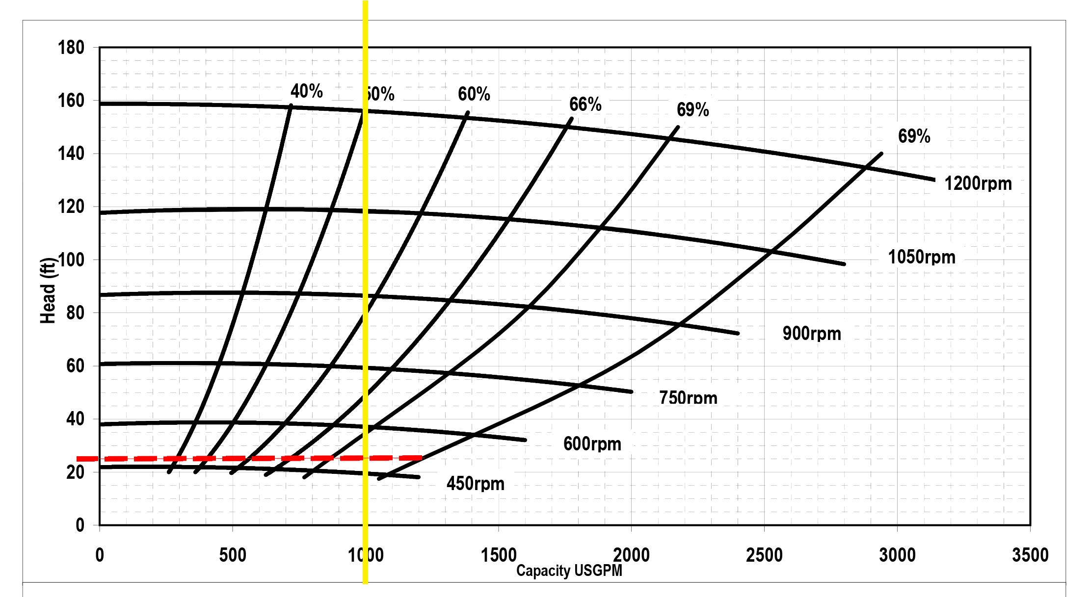
2. Identify the Pump's efficiency range
Efficiency is the ratio of useful power output to power input. The Pump curve shows the Pump’s efficiency as different operating points. The highest point of efficiency on the curve, referred to as the Best Efficiency Point (BEP), represents the optimal operating conditions for the Pump.
The graph depicting Total Dynamic Head and flow rate also features upward curving lines that illustrate efficiency (measured in percentage). The duty point of the Pump, as determined by the intersection of the Total Dynamic Head and flow rate, should fall within one of the listed efficiency ranges.
In the example below, the duty point of the Pump falls within the 69% efficiency range, which is considered an ideal selection.
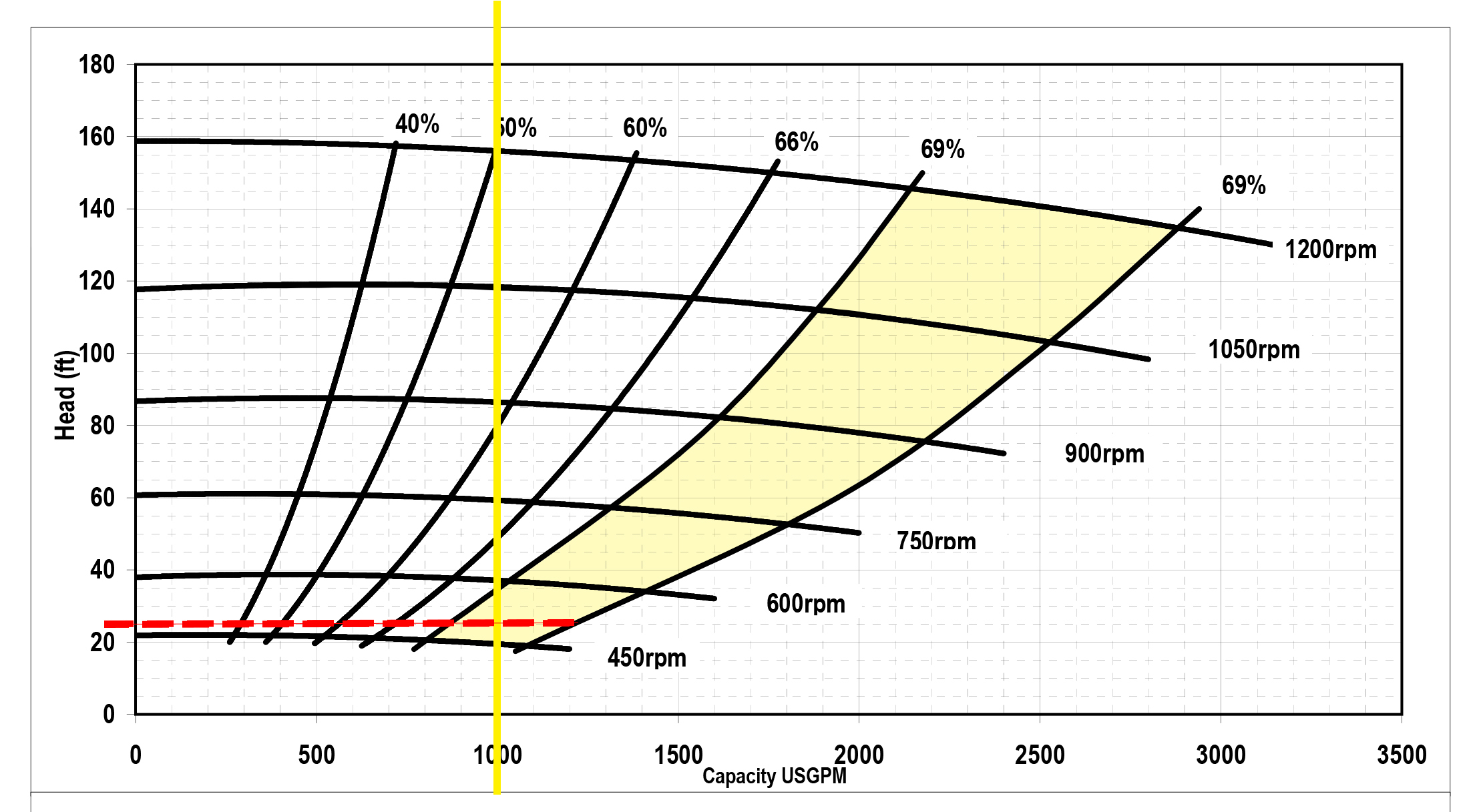
If the duty point falls on the right side of the shown efficiency curve, the Pump is generally considered out of range. With the same TDH, a greater flow rate could cause significant pumping issues. Avoid “operating on the right side of the curve” in most circumstances.
3. Identify the required Pump speed
The graph depicting Total Dynamic Head and flow rate also features horizontal curving lines that illustrate speed (measured in rpm). Speed is how fast the Pump needs to operate to meet the duty point. The duty point of the Pump, as determined by the intersection of the Total Dynamic Head and flow rate, should fall within one of the listed speed ranges.
In the example below, the Pump speed for the determined duty point is between 450 rpm and 600 rpm at approximately 500 rpm (shown in orange).
4. Determine the required horsepower
Using the information from this first graph, you can use the data on the next graph depicting power consumption and flow rate to determine the horsepower that will be required to operate the Pump at its duty point.
First, draw a vertical line through the known flow rate (shown in yellow), which, using the example above, is 1,000 gpm. Then, draw a horizontal line (shown in blue) at 500 rpm to the Y-axis, which is the operating speed as determined from the first graph. Where the horizontal line intersects with the Y-axis is the horsepower required, which in this example, is 10 HP.

How specific gravity affects Pump sizing and selection
Note that the power consumption graph depicts the required power to operate the Pump with only water; it does not show the impact of pumping a heavier slurry. Pumping material that is denser than water, such as an aggregate slurry, may require additional horsepower to move the same distance. The specific gravity of the slurry will be used to adjust the required horsepower for the application.
Since 12.3 isn’t a standard horsepower rating, round up to the next interval, which would be 15 in this case. Therefore, the horsepower required for the Pump to operate at its duty point with a sand and water slurry at 14% solids would be 15 HP.
How viscosity affects Pump sizing and selection
Viscosity is one of the more recognized physical properties of a fluid that influences the operation of a Pump. Viscosity measures the resistance to shear energy, such in a centrifugal Pump. Honey at room temperature exhibits high internal resistance to flow and is considered to have a high viscosity. A low viscosity liquid possesses a low internal resistance to flow, such as water at room temperature.
The effects of viscosity show up in calculating friction losses in a fluid process system and must be considered to make a good Pump selection. In general, a centrifugal Pump is suitable for low viscosity fluids since the pumping action generates high liquid shear. As the viscosity of the fluid increases, the flow rate is slightly reduced, with a more significant impact on the power draw of the Pump.
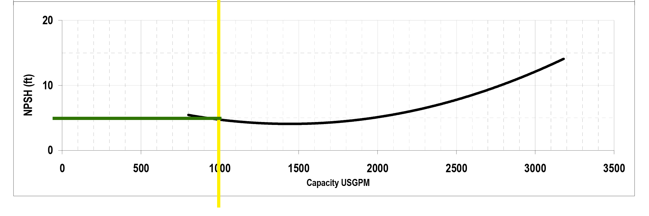
5. Determine the NPSHr
The Net Positive Suction Head required is depicted on the third graph. Draw vertical line (shown in yellow below) at the known flow rate, which from our example we know to be 1,000 gpm. At the point where the vertical line intersects the plot information, draw a horizontal line (shown in green below) to the Y-axis. For this example, the NPSHr is 5’ of pressure.
Pump curves can provide valuable information for selecting the right Pump for an application. They use existing application data from the Total Dynamic Head and flow rate to size the Pump, and to then find the speed and horsepower required to operate the Pump at its duty point within an ideal efficiency range. They also provide information to calculate the Net Positive Suction Head required, which is the minimum pressure above the suction line to avoid cavitation — the imploding of vapor bubbles within the Pump that can cause serious Pump issues.
By examining the Pump curve, users can determine the Pump’s performance at various flow rates and head conditions, which is crucial for selecting the right Pump for an application and for optimizing its operation for energy efficiency.


